
The Central Limit Theorem is such an important and fundamental theorem of probability and statistics that it pops up all over the place. You’ll see it mentioned in many articles around hypothesis testing, confidence intervals and more as the justification for using the normal distribution. It is one of the reasons that the normal distribution is so widely used and it’s worth taking time to really understand.
Let’s jump straight into its formal definition and we’ll use a few illustrations to help explain.
The Definition
The Central Limit Theorem states that, as the sample size N increases, the distribution of the sample means approaches a normal distribution, regardless of the distribution of the population.
Ok so what does this actually mean?
First, we’re talking about samples and populations. We have a population and we want to understand its mean. It’s normally not feasible to know the true mean of a population so we take a sample instead. The CLT says that if we take multiple samples of size N and then take the mean of each sample, if we then plot the means, we would see a normal distribution, provided each sample of N was big enough.
For example, say we want to understand the conversion rate of a webpage. The population theoretically could be said to be everyone who has used and will use that webpage. We can’t get this so instead we sample the performance of the page for a week. We monitor the page and randomly select multiple samples of 30 visitors each. From each group of 30 we calculate a conversion rate. The Central Limit Theorem says that the conversion rates plotted in a histogram will follow a normal distribution.
We illustrate this example with the drawing below.
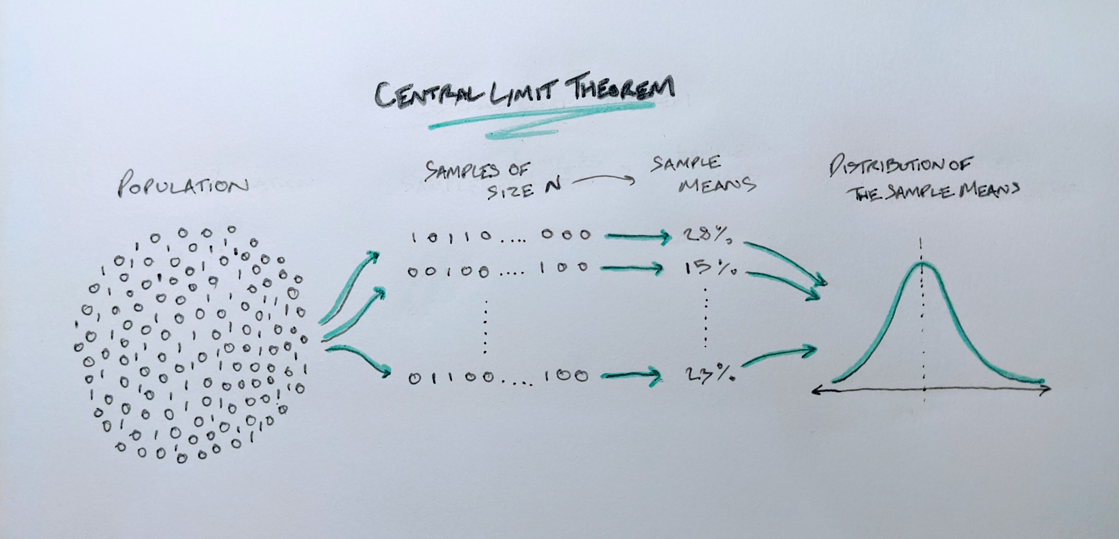 Handdrawn illustration of the Central Limit Theorem
Despite the population distribution being just a discrete distribution of 1s and 0s (a 1 signifying a purchase), when we take samples of size N, we see that the distribution of the sample mean approaches the classic bell curve associated with the normal distribution.
The CLT states that the sample means approximate a normal distribution as the sample size increases. It’s also sometimes stated that the Central Limit Theorem applies “for sufficiently large N”. So what sample size do we need before we can assume normality of the sample mean distribution? And why does it have to be large anyway? We’ll use Python to illustrate this.
An Illustration of the Theorem in Action
Here we see the theorem in action. We take four non-normal distributions and take samples of increasing sizes of N to see the Central Limit Theorem in effect. For each of the distributions, we start with 10,000 values. These are plotted as the black line in each graph and show the original distribution that we take samples from.
The shaded sections show the distribution of the sample means. For these, we take 1000 samples from each distribution for 4 different sample sizes: 5, 10, 20 and 50. This means that for each distribution we take 1000 samples where each sample contains 5 values. We get the mean of each sample of 5 and then plot the 1000 means (this is the blue shaded area). We then do the same again but with each sample containing 10 values, then the same for sample sizes 20 and 50. The number of values taken into each sample represents the sample size N that has to be sufficiently large in the Central Limit Theorem. We can see why in the plots below.
Code to produce plots
# Create the random samples
uniform = np.random.uniform(0, 1, 10000)
poisson = np.random.poisson(3, 10000)
binomial = np.random.binomial(1000, 0.5, 10000)
exponential = np.random.exponential(1, 10000)
distributions = {'Uniform': uniform,
                'Poisson': poisson,
                'Binomial': binomial,
                'Exponential': exponential}
n_sizes = [5, 10, 20, 50]

fig, axs = plt.subplots(2, 2, figsize=(10, 8), dpi=150)
# To loop over the subplots
axs = axs.ravel()

# Loop over the distributions and the subplots
for dist, axis in zip(distributions, range(4)):
    sns.kdeplot(distributions[dist], ax=axs[axis], color='black')
    # Loop over the sample sizes
    for n in n_sizes:
        sample_means = []
        for i in range(1000):
            # Loop over the 1000 samples
            sample_means.append(np.random.choice(distributions[dist], n).mean())
        sns.kdeplot(sample_means, shade=True, ax=axs[axis])
        axs[axis].set_title(dist)
fig.tight_layout()
plt.show();
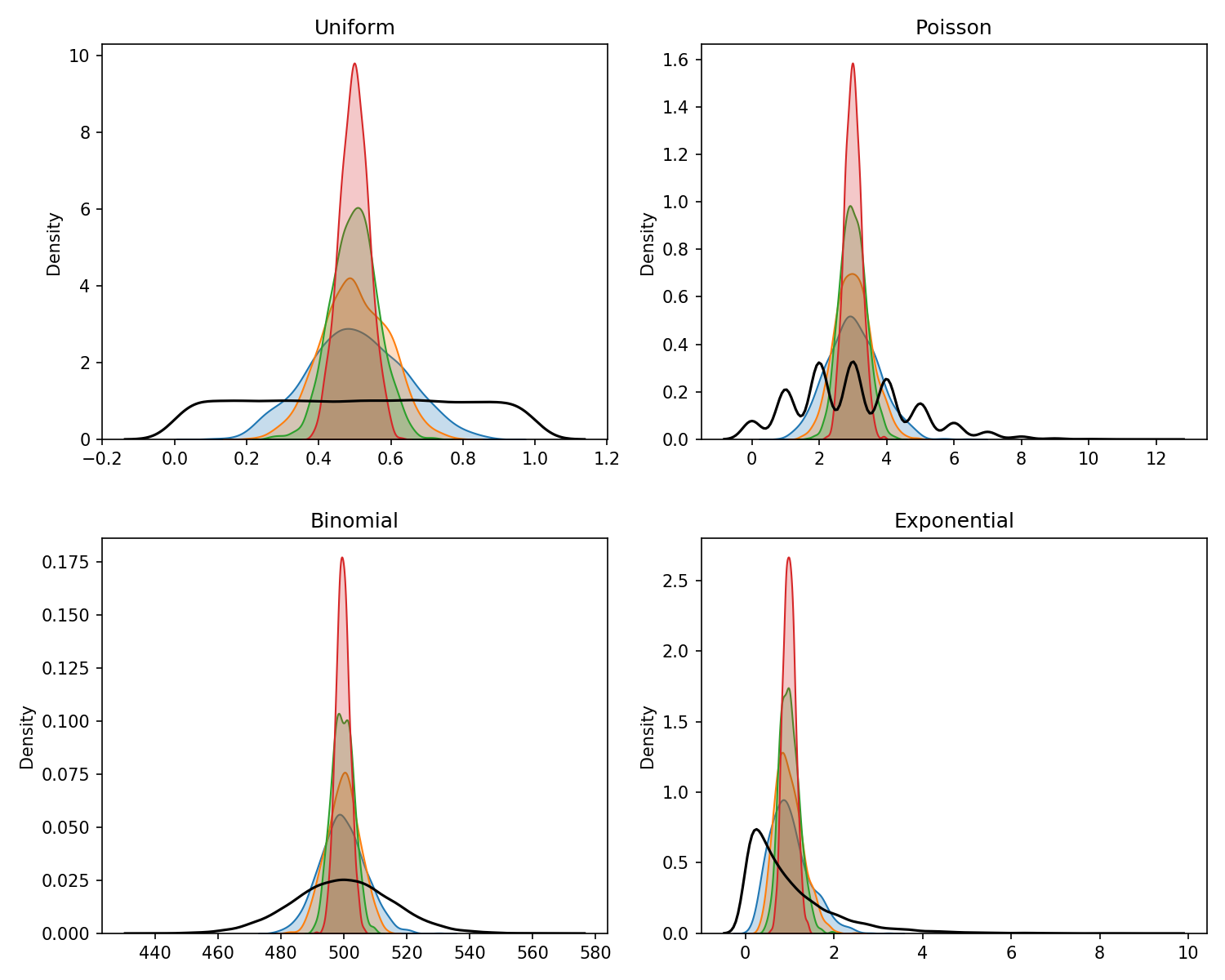 The underlying distribution for each plot is shown in black - the shaded plots show the distribution of the sample means for increasing samples of n
As the sample size increases from 5 to 50, we see that the distribution resembles a normal distribution more and more with it being centred around a central point with tails on either side. This is true for each of the four non-normal distributions showing the wonder of the CLT.
If you look closely you can see that some distributions start to approach a normal distribution quicker than others with the Binomial looking very close immediately with only a sample size of N=5 whereas the exponential distribution still shows a skew with N=20. This is why there is no magic sufficiently large N from which point the CLT kicks-in and we can assume normality, there are only rules of thumb. Generally, a sample size of 30 is widely used as a rule of thumb for what counts as sufficiently large N.
How is it Used in Practice?
In the examples mentioned already, we take 1000s of samples each with sample size N. However, in practice, we don’t have to take 1000s of samples of size N before we can assume they follow a normal distribution. In practice, we just take the one sample. Using the rule of thumb, if we have a sample of more than 30 values, we can model the mean of the sample using the normal distribution, opening up the possibility to perform hypothesis tests, create confidence intervals and more incredible tools in inferential statistcs available to normally distributed data.
Why is it Important?
I’ve already mentioned hypothesis tests a bunch of times and this is where I come across the CLT being mentioned most often. When analysing AB tests, we often use a Z-test. One of the assumptions of the Z-test is that the distribution of the test statistic (i.e. the conversion rate) can be approximated by a normal distribution. If our sample size is greater than 30, which it absolutely will be for any AB test, then we can forego the tedious normality checks that we would otherwise need to run. The same checks would be needed for t-tests, analysis of variance (ANOVA), Chi-squared tests and more if it were not for the CLT.
Another very important theorem in probability is the Law of Large Numbers (LLN) and it is crucial to the CLT. The LLN states quite simply that if we take a sample from a population, the mean of the sample will approach the true mean of the population the more samples we take. Put mathematically,
\(\bar{X} \to \mu\) as \(N \to \infty\) where \(\bar{X}\) is the sample mean and \(\mu\) is the population or true mean.
The LLN deserves its own article but I mention it here because it is this theorem and its role in the Central Limit Theorem that tells us that as the sample size increases, the accuracy of our sample mean estimate increases. For anyone who has ever analyse a hypothesis test, they will know that this is what we wait for. We wait until we have great enough precision in our sample mean estimates to show that the performance we have seen is extremely unlikely to have occurred under the null hypothesis.
Using the CLT, we can create a confidence interval from our sample mean and add more data to increase its precision giving us more confidence to make data-driven decisions.
To conclude, the Central Limit Theorem is one of the most important and fundamental theorems in statistics. It is well worth taking the time to understand and I hope that the next time you see the Central Limit Theorem casually thrown around as the cause for a normality assumption or thrown in for something else, you now understand why. Maybe you’ll also find ways to leverage the theorem to simplify aspects of your analysis and stop worrying about distributions and learn to love the theorem.


